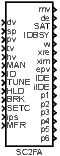
SC2FA – State controller for 2nd order system with frequency autotuner

Block SymbolLicensing group: AUTOTUNING

Function Description
The SC2FA block implements a state controller for 2nd order system (7.4) with frequency autotuner. It is well suited especially for control (active damping) of lightly damped systems ( $ξ < 0 . 1$ ). But it can be used as an autotuning controller for arbitrary system which can be described with sufficient precision by the transfer function

$F (s) = \frac{b_{1} s + b_{0}}{s^{2} + 2 ξ Ω s + Ω^{2}},$

(7.4)

where $Ω > 0$ is the natural (undamped) frequency, $ξ$ , $0 < ξ < 1$ , is the damping coefficient and $b_{1}$ , $b_{0}$ are arbitrary real numbers. The block has two operating modes: "Identification and design mode" and "Controller mode".

The "Identification and design mode" is activated by the binary input $ID = on$ . Two points of frequency response with given phase delay are measured during the identification experiment. Based on these two points a model of the controlled system is built. The experiment itself is initiated by the rising edge of the RUN input. A harmonic signal with amplitude uamp, frequency $ω$ and bias ubias then appears at the output mv. The frequency runs through the interval $⟨ wb, wf ⟩$ , it increases gradually. The current frequency is copied to the output w. The rate at which the frequency changes (sweeping) is determined by the cp parameter, which defines the relative shrinking of the initial period $T_{b} = \frac{2 π}{wb}$ of the exciting sine wave in time $T_{b}$ , thus

cp=wbω(Tb)=wbwbeγTb=e−γTb.<math xmlns="http://www.w3.org/1998/Math/MathML" display="block"><mrow> <msub><mrow><mi>c</mi></mrow><mrow><mi>p</mi></mrow></msub> <mo class="MathClass-rel">=</mo> <mfrac><mrow><mstyle class="text"><mtext class="texttt" mathvariant="monospace">wb</mtext></mstyle></mrow> <mrow><mi>ω</mi><mrow><mo class="MathClass-open">(</mo><mrow><msub><mrow><mi>T</mi></mrow><mrow><mi>b</mi></mrow></msub></mrow><mo class="MathClass-close">)</mo></mrow></mrow></mfrac> <mo class="MathClass-rel">=</mo> <mfrac><mrow><mstyle class="text"><mtext class="texttt" mathvariant="monospace">wb</mtext></mstyle></mrow> <mrow><mstyle class="text"><mtext class="texttt" mathvariant="monospace">wb</mtext></mstyle><msup><mrow><mi>e</mi></mrow><mrow><mi>γ</mi><msub><mrow><mi>T</mi></mrow><mrow><mi>b</mi></mrow></msub></mrow></msup></mrow></mfrac> <mo class="MathClass-rel">=</mo> <msup><mrow><mi>e</mi></mrow><mrow><mo class="MathClass-bin">−</mo><mi>γ</mi><msub><mrow><mi>T</mi></mrow><mrow><mi>b</mi></mrow></msub> </mrow></msup><mo class="MathClass-punc">.</mo> </mrow></math>

The cp parameter usually lies within the interval $cp \in ⟨ 0, 95; 1)$ . The lower the damping coefficient $ξ$ of the controlled system is, the closer to one the cp parameter must be.

At the beginning of the identification period the exciting signal has a frequency of $ω = wb$ . After a period of stime seconds the estimation of current frequency response point starts. Its real and imaginary parts are available at the xre and xim outputs. If the MANF parameter is set to 0, then the frequency sweeping is stopped two times during the identification period. This happens when points with phase delay of ph1 and ph2 are reached for the first time. The breaks are stime seconds long. Default phase delay values are $- 6 0^{\circ}$ and $- 12 0^{\circ}$ , respectively, but these can be changed to arbitrary values within the interval $(- 36 0^{\circ}, 0^{\circ})$ , where $ph1 > ph2$ . At the end of each break an arithmetic average is computed from the last iavg frequency point estimates. Thus we get two points of frequency response which are successively used to compute the controlled process model in the form of (7.4). If the MANF parameter is set to 1, then the selection of two frequency response points is manual. To select the frequency, set the input $HLD = on$ , which stops the frequency sweeping. The identification experiment continues after returning the input HLD to 0. The remaining functionality is unchanged.

It is possible to terminate the identification experiment prematurely in case of necessity by the input $BRK = on$ . If the two points of frequency response are already identified at that moment, the controller parameters are designed in a standard way. Otherwise the controller design cannot be performed and the identification error is indicated by the output signal $IDE = on$ .

The IDBSY output is set to 1 during the "identification and design" phase. It is set back to 0 after the identification experiment finishes. A successful controller design is indicated by the output $IDE = off$ . During the identification experiment the output iIDE displays the individual phases of the identification: $iIDE = - 1$ means approaching the first point, $iIDE = 1$ means the break at the first point, $iIDE = - 2$ means approaching the second point, $iIDE = 2$ means the break at the second point and $iIDE = - 3$ means the last phase after leaving the second frequency response point. An error during the identification phase is indicated by the output $IDE = on$ and the output iIDE provides more information about the error.

The computed state controller parameters are taken over by the control algorithm as soon as the SETC input is set to 1 (i.e. immediately if SETC is constantly set to on). The identified model and controller parameters can be obtained from the p1, p2, …, p6 outputs after setting the ips input to the appropriate value. After a successful identification it is possible to generate the frequency response of the controlled system model, which is initiated by a rising edge at the MFR input. The frequency response can be read from the w, xre and xim outputs, which allows easy confrontation of the model and the measured data.

The "Controller mode" (binary input $ID = off$ ) has manual ( $MAN = on$ ) and automatic ( $MAN = off$ ) submodes. After a cold start of the block with the input $ID = off$ it is assumed that the block parameters mb0, mb1, ma0 and ma1 reflect formerly identified coefficients $b_{0}$ , $b_{1}$ , $a_{0}$ and $a_{1}$ of the controlled system transfer function and the state controller design is performed automatically. Moreover if the controller is in the automatic mode and $SETC = on$ , then the control law uses the parameters from the very beginning. In this way the identification phase can be skipped when starting the block repeatedly.

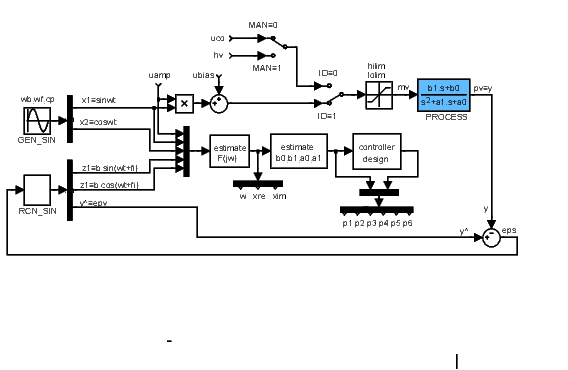
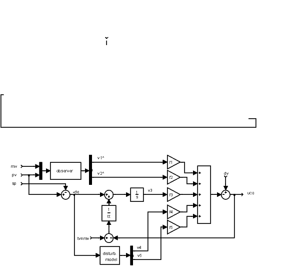
The diagram above is a simplified inner structure of the frequency autotuning part of the controller. The diagram below shows the state feedback, observer and integrator anti-wind-up. The diagram does not show the fact, that the controller design block automatically adjusts the observer and state feedback parameters $f 1, \dots, f 5$ after identification experiment (and $SETC = on$ ).

The controlled system is assumed in the form of (7.4). Another forms of this transfer function are

$F (s) = \frac{(b_{1} s + b_{0})}{s^{2} + a_{1} s + a_{0}}$

(7.5)

and

$F (s) = \frac{K_{0} Ω^{2} (τ s + 1)}{s^{2} + 2 ξ Ω s + Ω^{2}} .$

(7.6)

The coefficients of these transfer functions can be found at the outputs p1,...,p6 after the identification experiment ( $IDBSY = off$ ). The output signals meaning is switched when a change occurs at the ips input.

Inputs

dv	Feedforward control variable	Double (F64)
sp	Setpoint variable	Double (F64)
pv	Process variable	Double (F64)
tv	Tracking variable	Double (F64)
hv	Manual value	Double (F64)
MAN	Manual or automatic mode	Bool
	off .. Automatic mode on ... Manual mode
ID	Identification or controller operating mode	Bool
	off .. Controller mode on ... Identification and design mode
TUNE	Start the tuning experiment (off $\to$ on), the exciting harmonic signal is generated	Bool
HLD	Stop frequency sweeping	Bool
BRK	Termination signal	Bool
SETC	Flag for accepting the new controller parameters and updating the control law	Bool
	off .. Parameters are only computed on ... Parameters are accepted as soon as computed off $\to$ on One-shot confirmation of the computed parameters
ips	Switch for changing the meaning of the output signals	Long (I32)
	0 .... Two points of frequency response p1 … frequency of the 1st measured point in rad/s p2 … real part of the 1st point p3 … imaginary part of the 1st point p4 … frequency of the 2nd measured point in rad/s p5 … real part of the 2nd point p6 … imaginary part of the 2nd point 1 .... Second order model in the form (7.5) p1 … $b_{1}$ parameter p2 … $b_{0}$ parameter p3 … $a_{1}$ parameter p4 … $a_{0}$ parameter 2 .... Second order model in the form (7.6) p1 … $K_{0}$ parameter p2 … $τ$ parameter p3 … $Ω$ parameter in rad/s p4 … $ξ$ parameter p5 … $Ω$ parameter in Hz p6 … resonance frequency in Hz 3 .... State feedback parameters p1 … $f_{1}$ parameter p2 … $f_{2}$ parameter p3 … $f_{3}$ parameter p4 … $f_{4}$ parameter p5 … $f_{5}$ parameter
MFR	Generation of the parametric model frequency response at the w, xre and xim outputs (off $\to$ on triggers the generator)	Bool

Outputs

mv	Manipulated variable (controller output)	Double (F64)
de	Deviation error	Double (F64)
SAT	Saturation flag	Bool
	off .. The controller implements a linear control law on ... The controller output is saturated
IDBSY	Identification running	Bool
	off .. Identification not running on ... Identification in progress
w	Frequency response point estimate - frequency in rad/s	Double (F64)
xre	Frequency response point estimate - real part	Double (F64)
xim	Frequency response point estimate - imaginary part	Double (F64)
epv	Reconstructed pv signal	Double (F64)
IDE	Identification error indicator	Bool
	off .. Successful identification experiment on ... Identification error occurred
iIDE	Error code	Long (I32)
	101 .. Sampling period too low 102 .. Error identifying one or both frequency response point(s) 103 .. Manipulated variable saturation occurred during the identification experiment 104 .. Invalid process model
p1..p6	Results of identification and design phase	Double (F64)

Parameters

ubias	Static component of the exciting harmonic signal	Double (F64)
uamp	Amplitude of the exciting harmonic signal $⊙$ 1.0	Double (F64)
wb	Frequency interval lower limit [rad/s] $⊙$ 1.0	Double (F64)
wf	Frequency interval upper limit [rad/s] $⊙$ 10.0	Double (F64)
isweep	Frequency sweeping mode $⊙$ 1	Long (I32)
	1 .... Logarithmic 2 .... Linear (not implemented yet)
cp	Sweeping rate $↓$ 0.5 $↑$ 1.0 $⊙$ 0.995	Double (F64)
iavg	Number of values for averaging $⊙$ 10	Long (I32)
alpha	Relative positioning of the observer poles (in identification phase) $⊙$ 2.0	Double (F64)
xi	Observer damping coefficient (in identification phase) $⊙$ 0.707	Double (F64)
MANF	Manual frequency response points selection	Bool
	off .. Disabled on ... Enabled
ph1	Phase delay of the 1st point in degrees $⊙$ -60.0	Double (F64)
ph2	Phase delay of the 2nd point in degrees $⊙$ -120.0	Double (F64)
stime	Settling period [s] $⊙$ 10.0	Double (F64)
ralpha	Relative positioning of the observer poles $⊙$ 4.0	Double (F64)
rxi	Observer damping coefficient $⊙$ 0.707	Double (F64)
acl1	Relative positioning of the 1st closed-loop poles couple $⊙$ 1.0	Double (F64)
xicl1	Damping of the 1st closed-loop poles couple $⊙$ 0.707	Double (F64)
INTGF	Integrator flag $⊙$ on	Bool
	off .. State-space model without integrator on ... Integrator included in the state-space model
apcl	Relative position of the real pole $⊙$ 1.0	Double (F64)
DISF	Disturbance flag	Bool
	off .. State space model without disturbance model on ... Disturbance model is included in the state space model
dom	Disturbance model natural frequency $⊙$ 1.0	Double (F64)
dxi	Disturbance model damping coefficient	Double (F64)
acl2	Relative positioning of the 2nd closed-loop poles couple $⊙$ 2.0	Double (F64)
xicl2	Damping of the 2nd closed-loop poles couple $⊙$ 0.707	Double (F64)
tt	Tracking time constant $⊙$ 1.0	Double (F64)
hilim	Upper limit of the controller output $⊙$ 1.0	Double (F64)
lolim	Lower limit of the controller output $⊙$ -1.0	Double (F64)
mb1p	Controlled system transfer function coefficient $b_{1}$	Double (F64)
mb0p	Controlled system transfer function coefficient $b_{0}$ $⊙$ 1.0	Double (F64)
ma1p	Controlled system transfer function coefficient $a_{1}$ $⊙$ 0.2	Double (F64)
ma0p	Controlled system transfer function coefficient $a_{0}$ $⊙$ 1.0	Double (F64)

[Previous] [Back to top] [Up] [Next]